Authors:
In this third post we pick one particular operation, filter, and look under the hood to see how the XOR DataFrame API allows the analyst to write efficient data workflow without having to worry about the data stacking, locality, and visibility.
Filtering operation
In a data analysis workflow, one will often want to remove, or filter out, certain rows of the dataset to focus on a subset of samples. For example, the analyst might only be interested in sensor data coming from a particular factory. The inputs to this operation are the predicate column, a column of boolean values that indicates which row should be kept (True) or discarded (False), and the XOR DataFrame to be filtered. This latter must have the same number of rows as the predicate column.
We use the same setup as in the blog posts part 1 and part 2. Let’s see how different data stackings can lead to different flows of computations when executing the filter operation. In all cases, you will see that we might chain several local and/or MPC computations to obtain the desired result.
Case 1. Only local computation
Let’s assume our analyst Rose wants to only keep rows with run_id > 8912 from the sensor data of the German factory.
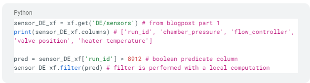
The input DataFrame sensor_DE_xf is fully owned by a single player and is plaintext. In this case, the most efficient is to use a local computation to filter rows. This amounts to using the loc method from the popular Python library Pandas.
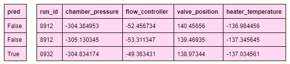
Table 1. Plaintext datasets owned solely by the German factory
Case 2. The predicate column allows local computation
Rose could also perform the same filtering but on the aggregated sensor data from both factories. As pred is available locally to each compute party (see below why), we use a local computation to generate a vector of the row indices to be kept. Then execute a multiparty computation that extracts the correct rows from sensor_agg_xf. This is analogous to iloc in Pandas, though it is executed in an MPC setting.
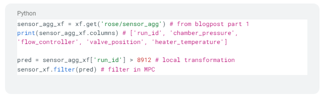
The XOR DataFrame sensor_agg_xf was the result of a groupby(by=‘run_id’, on=sensor_names).mean() operation, see blog 1. The visibility of the by column is plaintext and it is owned by all players who participated in the computation, i.e. the German and US factories (this is color coded in yellow below). Which means that each player has a copy of the “yellow data”, and we can run local computations. The on columns have secret-share visibility (in green below), meaning that each player has a share of the data but does not see the actual value. Only MPC computations are possible on secret-share data.
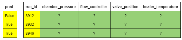
Table 2. Plaintext columns (yellow) and secret-shared columns (green) owned by the same players
Case 3. Only MPC
Let’s look at a more complex data stacking example. Rose wants to keep the rows of joined_xf from blog 2, having a target value y < 100. The input DataFrame joined_xf is the result of the join between the metrology and aggregated sensor datasets: join([metrology_xf, sensor_agg_xf], on=‘run_id’).
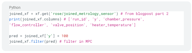
As shown in Table 3, the y and pred records are plaintext and are either owned by the German (pink) or US (blue) factory. Because the pred column is owned by different players, only MPC computation is possible.
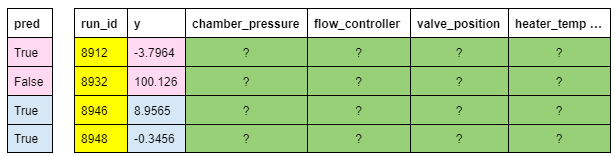
Table 3. Plaintext predicate column owned by different players (pink and blue)
In this case we perform an oblivious sort on the pred column, which orders all the 0 entries (False) before the 1s (True). We then apply the same private sorting permutation to joined_xf, count the number of 1s in pred, say N, and keep the last N rows. Of course everything is done in MPC without revealing the actual data, including the row indices to be retained.
To generate new DataFrames, the computation backend must know the dimensions of every dataset involved. As such, the number of rows N of the output DataFrame must be revealed to the DataFrame Interpreter. This is done automatically and is transparent to the user.
Conclusion
By using the DataFrame API, the analyst can execute complex data analysis tasks that require the chaining of many local and/or MPC computations in the background. Information about dataset stacking, visibility, and location is taken into account to choose the most efficient graph of computations for the desired result. From the analyst’s perspective, these concerns are abstracted away, and she is presented with an interface that contains operations she is used to: filter, join, groupby, etc. This streamlines the data analysis and helps produce insights about distributed datasets quickly by leveraging the power of MPC computations.