Neuroimaging Based Diagnosis of Alzheimer’s Disease Using Privacy-Preserving Machine Learning (Part 2)

Authors: Prof. Bogdan Draganski (Director, LREN), Dr. Ferath Kherif (Vice Director, LREN), Claudio Calvaruso (Technical Account Manager, Inpher) and Dr. Dimitar Jetchev (CTO, Inpher)

Editors Note: This is the second in a series of articles that LREN – CHUV and Inpher are jointly publishing to show how privacy-preserving machine learning allows for neuroimaging-based diagnosis of Alzheimer’s disease that is readily applicable in a federated network. Read part 1 here

Introduction

In part 1 of this blog post, we shared how the latest advancements in MRI imaging and Statistical Parametric Mapping (SPM) can benefit from the recent developments in Privacy-Enhancing Technologies (PETs), Privacy-Preserving Machine Learning (PPML) and Privacy-Preserving Federated Learning (PPFL) to address challenges in understanding the mechanisms (from a researcher’s perspective) in the early diagnosis of Alzheimer’s Disease (from a clinical perspective): 

• Researchers’ perspective: Identifying relevant biological variables including regional changes in brain volume associated with the pathologies of AD and other dementias to understand the mechanisms underlying Alzheimer’s disease

• Clinicians’ perspective: individual diagnostics estimating accurate risk score and propensity of neuromodulatory treatment for a given patient to support better diagnosis

In part 2 of the blog post, we describe two specific simple models, a linear and a logistic regression model, addressing each of the two aspects above and the workflows needed for the training across data coming from multiple private data sources (hospitals, private radiology labs or research institutes) using a combination of SPM tools for local processing and Inpher’s XOR Secret Computing© Platform for PPML. 

Training Privacy-Preserving Linear Regression Models

Linear regression is a basic supervised learning method for modeling the relationship between a scalar response and one or more explanatory variables (features) where one wants to estimate the coefficient of the slope that best fits the input training data. 

In our scenarios, the individuals’ brain MRI scans are first mapped at the voxel level to the Jacobian determinant template of the SPM tools (described in part 1 of this post)  to quantify temporal grey matter changes. This preprocessing is local to each private data source. One then uses generalized linear models and hypothesis testing across a set of healthy controls (HC) and Alzheimer disease subjects (AD) to distinguish if these temporal expansions (or contractions) are due to Alzheimer’s disease or regular temporal changes due to aging.

More precisely, it is defined as matrix Y (the dependent variable matrix) of size N x 20,000 where N is the total number of patients across all data sources and the 20,000 columns correspond to the 20,000 voxels of the images. Each row of this matrix corresponds to the voxel values of the SPM-preprocessed Jacobian template for a given patient (HC or AD patient) and each column corresponds to a particular voxel in the standard stereotaxic space. 

The goal is to compute a linear model for each column expressing the voxel value as a linear function of certain feature values. The features correspond to the columns of a feature matrix referred to as a design matrix. The rows of the design matrix correspond to the subjects (both HC and AD). Figure 1 represents a typical design matrix (where N_samples, in this case, correspond to the total number of patients). The first column (consisting of 1’s) is optional and may represent the intercept in the regression model. The second (binary) column is the characteristic vector of the healthy controls – the binary entry corresponding to a sample (or patient) is 1 if the patient is in HC and 0 otherwise. Similarly, the third one is the characteristic vector of the clinically labeled Alzheimer patients – the binary entry corresponding to a patient is 0 if the patient is in HC and 1 if the patient has been diagnosed with AD. We can also represent features such as age, gender, race and other phenotyping features as illustrated in Figure 2.  

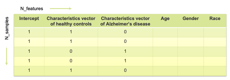
Figure 1: Example Feature Matrix (Product Matrix)

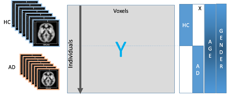
Figure 2: Fitting a Linear Regression Model per Voxel

For each voxel of the image (column of the matrix Y), the voxel value y is expressed in terms of the above design matrix X as  

y= X .(β₀, β_HC, β_AD, β_AGE, β_GENDER, β_RACE)+ e.

Therefore, about 20,000 linear regression parameters are obtained, one for each voxel. Here, β₀ is the intercept, β_HC, β_AD, β_AGE, β_GENDER, β_RACE are the coefficients corresponding to HC, AD, age, gender, and race, respectively. The null hypothesis is β_HC =  β_AD. Rejecting the null hypothesis (rejecting values less than or equal) means that the particular voxel is functionally related to Alzheimer’s (see Figure 3) 

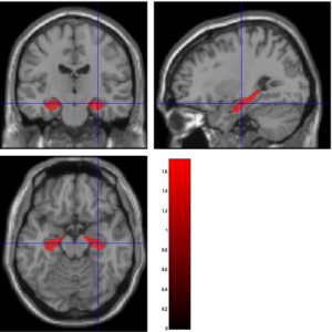
Figure 3: Linear Hypothesis Test (LHT) to identify voxels where HC>AD

Privacy-Preserving Training of Diagnosis Models for Alzheimer’s Disease

In the second scenario (clinicians’ setting), the goal is to build a tool for early and accurate diagnosis of Alzheimer’s Disease. Here, the role of the voxel matrix described in the previous section changes – it now becomes the feature matrix itself, or the independent variables matrix used to predict the risk score for a patient. In other words, the input features are the voxel values of an SPM preprocessed (via the Jacobian determinant template) MRI image of a new subject together with other data for that subject, such as clinical phenotyping data biomarkers. The output is an estimate of the risk of Alzheimer’s disease for the given subject.   

In order to obtain a meaningful and unbiased prediction model, the local training datasets available in a single hospital alone are insufficient. First and foremost, a single hospital is unlikely to provide enough subjects for the model training. Second, even if one were able to aggregate data from several large hospitals, the training data might still be biased since most of the MRI scans generated at these locations are not scans of healthy controls, hence the need to include more diverse data sources such as private clinics and radiology labs.  Finally, in most cases, patients’ MRI scans and age features do not follow identical distributions across the distinct private data sources. 

To overcome this challenge, Inpher’s XOR Platform is leveraged, particularly XOR MPC (Multi-Party Computation) for PPML and XOR Federated Learning with MPC for secure aggregation for PPFL (for better scalability and model complexities). This enables the training of highly accurate and precise models by using all the available data in a privacy-preserving way. In addition, the PPFL approach could enable training highly accurate complex deep learning models as well.

Logistic Regression Models

The most basic technique to address this problem is logistic regression, though it is not the only one. There has been progress using more advanced supervised learning methods such as Support Vector Machines (SVMs) or deep neural network models among others. Logistic regression is a supervised learning method that models the probability of a binary class prediction using a logistic function such as the sigmoid function. In our particular problem, the larger the probability value, the higher the risk of Alzheimer’s disease is for the patient. As in the researchers’ setting, the training data contains samples from both HC and AD patients. The feature matrices have multiple columns corresponding to each of the voxel values for each sample as well as the other features (e.g., age, gender, race). As the total number of voxels per preprocessed MRI image is 20,000, the model has at least 20,000 features and is therefore very complex to train in real-time. Since not all voxels are relevant to Alzheimer’s disease, one can use various dimensionality reduction techniques to reduce the model complexity. 

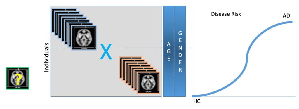
Figure 4: Estimating a Patient’s AD Risk score using Logistic Regression Model

Dimensionality Reduction Methods

There are three major dimensionality reduction techniques that one can use: 

1. Principal Component Analysis (PCA)

2. Prior spatial knowledge from an Atlas

3. Prior knowledge from the linear regression model in the previous section

The first approach is based on singular value decomposition (SVD) and needs a privacy-preserving algorithm. With the Inpher XOR Platform, data scientists are able to run such computations using secret-shared data. 

The second approach relies on prior spatial knowledge from an Atlas indicating what areas of the brain might be associated with AD. Examples of such Atlases are the Neuromorphometrics atlas released by “MICCAI 2012 Grand Challenge and Workshop on Multi-Atlas Labeling” (www.neuromorphometrics.com). 

The third approach uses the functional areas (voxels) identified to be statistically relevant to an Alzheimer’s Disease patient via the method in the previous section. It can be viewed as prior knowledge. If one chooses this approach, it is important to ensure independent datasets are used for the supervised training of the two models in order to avoid model biases. 

For the purpose of our simple model, here the first approach is chosen, that is, privacy-preserving PCA with Inpher’s XOR Platform.

Workflow for Training the Alzheimer’s Disease Logistic Regression Model

Figure 5 below explains the entire workflow for training the Alzheimer’s Disease logistic regression model. The MRI images for both the HC and AD cohorts are preprocessed with SPM locally at each hospital, private radiology lab or research institute. The output of the preprocessing are the voxel matrices X1, X2 and X3 (with the additional extra features). These matrices are large (have 20,000 columns) and they need to be vertically stacked to assemble the training dataset. 

One can first ingest the three matrices into the XOR Platform by letting each party secret share them among the three parties. Those can be then used with the XOR PCA functionality to obtain dimension-reduced feature matrix (a matrix with about 200 columns) secret shared among the three compute nodes. Lastly, these secret shares, together with the secret shared labels, are used to run the XOR logistic regression function to compute the final model. 

The output model can be kept “secret” to securely compute the class predictions and the positive class probability vector using a new MRI scan. Alternatively, it can be revealed to the data analyst or to any party that should have access to it and that should perform the predictions in plaintext, e.g., by instantiating a scikit-learn logistic regression classifier with the secretly trained model. 

The final quality assessment of the prediction on the test dataset can be done without revealing the predicted probabilities. This can be accomplished using the privacy-preserving: Confusion Matrix, Precision/Recall/F1 Score, and AUC functions available in the XOR Platform.

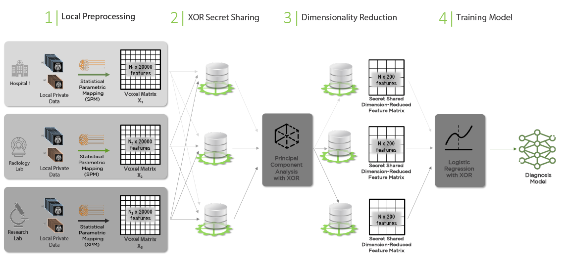
Figure 4: SPM with XOR MPC Workflow for Training Diagnosis Model

In cases where the goal is to derive the probability of more than one predictor at a time, then multilevel logistic regression is ideal. However, while this method could allow clinicians to draw a  better conclusion, the model’s quality, accuracy and reproducibility are highly dependent on the size and representativeness of the sample data. 

Inpher developed a federated approach that incorporated partial observations captured across multiple computing parties and built a high-level inference model based on multilevel Bayesian modeling to overcome these shortcomings. Intrinsically, the Bayesian Model comparisons scheme allows the comparison of the accuracy of specific models according to real-world data. Although the model was implemented with “privacy-by-design” principles, where only model parameters are exchanged between the computing parties, there were no explicit methods for protecting these parameters, such as encryption.

Conclusion 

In order to identify Alzheimer’s disease effectively,  it is necessary to have an unbiased prediction model. Unfortunately, if the training uses data available only at the hospital, the model can skew, since most of the samples are AD patients. Hence, having access to diverse data sources such as private clinics, radiology labs, and even pharmaceutical companies while safeguarding patient privacy is critical to building great predictive models. 

This blog describes how AI researchers and clinicians could leverage the sensitive data from multiple parties to build linear and logistic regression models using MPC in the XOR Platform. The next blog will provide a step-by-step python notebook walk-through example in order to demonstrate the real-world application for building these models with sensitive healthcare data.

Get started with privacy-preserving machine learning and experience what it’s like to build models by securely leveraging sensitive data from various sources.